Recently, I graduated from Udacity Robotics Software Engineer Nano Degree Program. Here are the links of my projects and certification. This post is the note that I took during learning process.
Gazebo
gazebo = gzserver + gzclient
Gazebo Server
- Responsible for parsing the description file related to scene/objects
- Can launch independently by
gzserver
Gazebo Client
- Provide graphic client that connects to gzserver
- Render the simulation scene
- Can run independently by
gzclient(waste if no gzserver)
World
1
gazebo <yourworld>.world
Formatted in SDF (Simulation Description Format):
1
2
3
4
5
6
7
8
9
10
11
12
13
14
15
16
17
18
19
20
21
22
23
24
25
<?xml version="1.0" ?>
<sdf version="1.5">
  <world name="default">
    <physics type="ode">
      ...
    </physics>

    <scene>
      ...
    </scene>

    <model name="box">
      ...
    </model>

    <model name="sphere">
      ...
    </model>

    <light name="spotlight">
      ...
    </light>

  </world>
</sdf>
Model
Include model in world
1
2
3
<include>
  <uri>model://model_file_name</uri>
</include>
Env Var
eg: GAZEBO_MODEL_PATH
Plugin
- Interactive with the world
- Can be loaded from cmd or added to world SDF
Example:
hello.cpp
1
2
3
4
5
6
7
8
9
10
11
12
13
14
15
16
17
18
19
#include <gazebo/gazebo.hh>

namespace gazebo {
    class WorldPluginMyRobot : public WorldPlugin {
      public:
        // Constructor
        WorldPluginMyRobot() : WorldPlugin() {
            printf("Hello World!\n");
        }

        // Mandatory
        void Load(physics::WorldPtr _world, sdf::ElementPtr _sdf) {

        }

    };

    GZ_REGISTER_WORLD_PLUGIN(WorldPluginMyRobot)
}
CMakeLists.txt
1
2
3
4
5
6
7
8
9
cmake_minimum_required(VERSION 2.8 FATAL_ERROR)

find_package(gazebo REQUIRED)
include_directories(${GAZEBO_INCLUDE_DIRS})
link_directories(${GAZEBO_LIBRARY_DIRS})
list(APPEND CMAKE_CXX_FLAGS "${GAZEBO_CXX_FLAGS}")

add_library(hello SHARED script/hello.cpp)
target_link_libraries(hello ${GAZEBO_LIBRARIES})
Export Plugin Path (optional)
1
export GAZEBO_PLUGIN_PATH=${GAZEBO_PLUGIN_PATH}:/home/workspace/myrobot/build
1
2
3
4
...
<world name="default">
    <plugin name="hello" filename="libhello.so"/>
...
RViz
- stands for ROS Visualization (Gazebo is a physics simulator)
- can visualize any type of sensor data (can be live-stream or bagfile)
1
roscore
1
2
3
# run rviz node in rviz pkg
# rosrun package_name executable_name
rosrun rviz rivz
ROS
History
- 2000s Stanford AI Lab
- 2007 Willow Garage startup
- 2013 Open Source Robotics Foundation
Topic vs. Service
Topic
-
massage passing through subscriber / publisher
-
define mesaage type in
.msgfile, i.e.: /msg/xxx,msg1 2 3
fieldtype1 fieldname1 fieldtype2 fieldname2 fieldtype3 fieldname3
-
Publisher C++ format
1
2
// queue_size: can store msg until being sent; exceeding will drop oldest
ros::Publisher pub1 = n.advertise<message_type>("/topic_name", queue_size);
-
Subscriber C++ format
1
ros::Subscriber sub1 = n.subscribe("/topic_name", queue_size, callback_function);
-
Service
-
Service: massage passing through request / response
-
define message type in
.srvfile, i.e: /srv/xxx.srv1 2 3 4 5 6 7 8 9 10 11 12 13
#request constants int8 FOO=1 int8 BAR=2 #request fields int8 foobar another_pkg/AnotherMessage msg --- #response constants uint32 SECRET=123456 #response fields another_pkg/YetAnotherMessage val CustomMessageDefinedInThisPackage value uint32 an_integer
-
Server c++ format
1
ros::ServiceServer service = n.advertiseService(`service_name`, handler);
-
Client c++ format
1
ros::ServiceClient client = n.serviceClient<package_name::service_file_name>("service_name");
-
Client call Server on Command Line
1
rosservice call service_name “request”
-
Turtlesim Example
Start nodes
1
2
# Master Process
roscore
1
rosrun turtlesim turtlesim_node
1
rosrun turtlesim turtle_teleop_key
List all active nodes
1
rosnode list
/rosout: launched by roscore. It subscribes to the standard /rosout topic which all nodes send log messages./teleop_turtle: keyboard teleop node/turtlesim: node name for turtlebot_sim node
List all topic
1
rostopic list
/rosout-
/rosout_agg: aggregated feed of messages -
/turtle1/cmd_vel: velosity cmds -
/turtle1/color_sensor: readings from the sensor are published to this topic /turtle1/pose: pose and orientation of turtle are published to this topic
Get topic info
1
rostopic info /turtle1/cmd_vel
-
Type: geometry_msgs/Twist
- Publishers:
- /teleop_turtle (http://jinux:38441/)
- Subscribers:
- /turtlesim (http://jinux:38975/)
Get message info
1
rosmsg info geometry_msgs/Twist
1
2
3
4
5
6
7
8
geometry_msgs/Vector3 linear
  float64 x
  float64 y
  float64 z
geometry_msgs/Vector3 angular
  float64 x
  float64 y
  float64 z
Edit ros msg
1
rosed geometry_msgs Twist.msg
1
2
3
# This expresses velocity in free space broken into its linear and angular parts.
Vector3  linear
Vector3  angular
Echo message on a topic
Listen to a topic
1
rostopic echo /turtle1/cmd_vel
URDF
-
Unified Robot Description Format
-
XML markup language
1
2
3
4
5
6
7
8
9
10
11
12
13
14
15
16
17
18
19
20
21
22
23
<?xml version="1.0"?>
<robot name="two_link_robot">
  <!--Links-->
  <link name="link_1">
    <visual>
      <geometry>
        <cylinder length="0.5" radius="0.2"/>
      </geometry>
    </visual>
  </link>
  <link name="link_2">
    <visual>
      <geometry>
        <box size="0.6 0.1 0.2"/>
      </geometry>
    </visual>
  </link>
  <!--Joints-->
  <joint name="joint_1" type="continuous">
    <parent link="link_1"/>
    <child link="link_2"/>
  </joint>
</robot>
Catkin
Workspace
A top-level directory where you build, install and modify catkin packages
Create a package:
Step 1: Create a catkin workspace and a sub directory
1
mkdir -p ~/workspace/catkin_ws/src
Step 2: Navigate to source directory
1
cd ~/workspace/catkin_ws/src
Step 3: Initialize the catkin workspace
1
catkin_init_workspace
Step 4: Build
1
2
cd ..
catkin_make
Package
A directory might contain
- CMakeLists.txt
- package.xml
- source code
- libraries
- database
- more …
Clone simple_arm example:
1
2
cd ~/workspace/catkin_ws/src/
git clone -b first_interaction https://github.com/udacity/RoboND-simple_arm/ simple_arm
Build the simple_arm package
1
2
cd ..
catkin_make
Create a catkin package:
1
2
3
cd ~/workspace/catkin_ws/src
# catkin_create_pkg <your_package_name> [dependency1 dependency2 …]
catkin_create_pkg first_package
Roslaunch
- launch ROS Master and multiple nodes
- Set default parameter on parameter server
- Auto re-spawn processes that have died
1
2
3
4
5
6
7
cd ~/workspace/catkin_ws/
catkin_make

# source devel/setup.zsh if you are in zsh
source devel/setup.bash

roslaunch simple_arm robot_spawn.launch
Rosdep
- check package’s missing dependencies
- download and install them
1
2
3
4
# must be sourced with source devel/setup.bash
rosdep check <package name>

rosdep install -i <package name>
Localization
Algorithms
- Extended Kalman Filter (EKF)
- Markov Localization
- Grid Localization
- Monte Carlo Localization (MCL)
Problems
- Position Tracking (easiest) – AKA Local Localization
- Know init pose
- Estimate pose as moving
- Global Localization
- Unknown init pose
- Determine pose relative to the ground truth map
- Kidnapped Robot (most difficult)
- Similar to Global Localization but may be kidnapped
- Teach itself to recover and correctly relocate
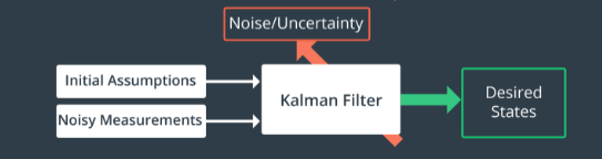
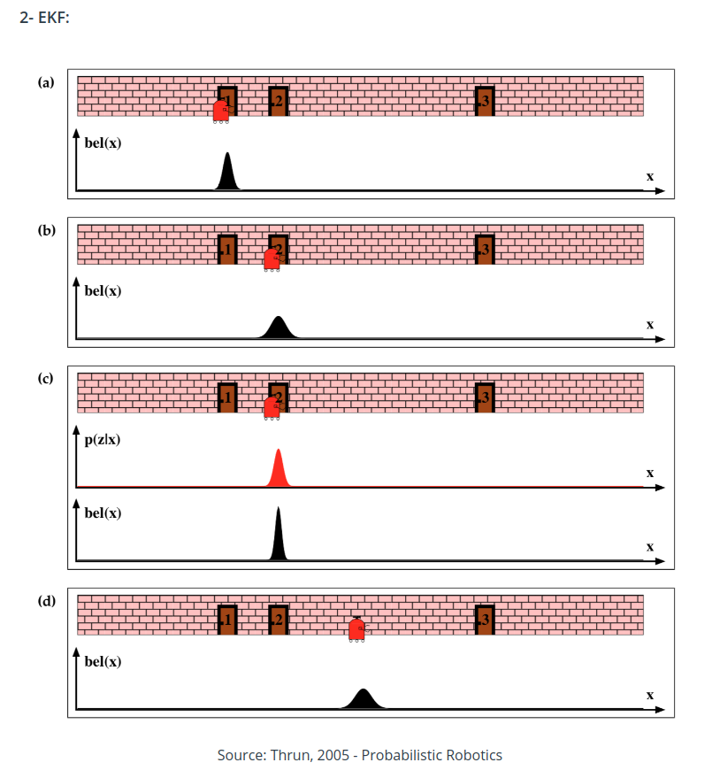
Kalman Filter
The Kalman Filter can only be applied to states that are represented by a Gaussian distribution.
Common Types
- KF - linear
- Extended Kalman Filter: EKF - nonlinear
- Unscented Kalman Filter: UKF - highly nonlinear
1D Gaussian
Formulas
The probability that a random variable, x, will take a value between $x_1$ and $x_2$ is given by the integral of the function from $x_1$ to $x_2$.
$p(x_1 < x < x_2) = \int_{x_1}^{x_2} f_x(x)dx$
Mean: $\mu$
Variance: $\sigma^2$
Gaussian Distribution Formula
$p(x) = \frac{1}{\sigma\sqrt{2\pi}}e^{-\frac{(x-\mu)^2}{2\sigma^2}}$
$\int p(x)dx = 1$
Variable Naming Conventions
- $x_t:state$
- $z_t: measurement$
- $u_t: control action$
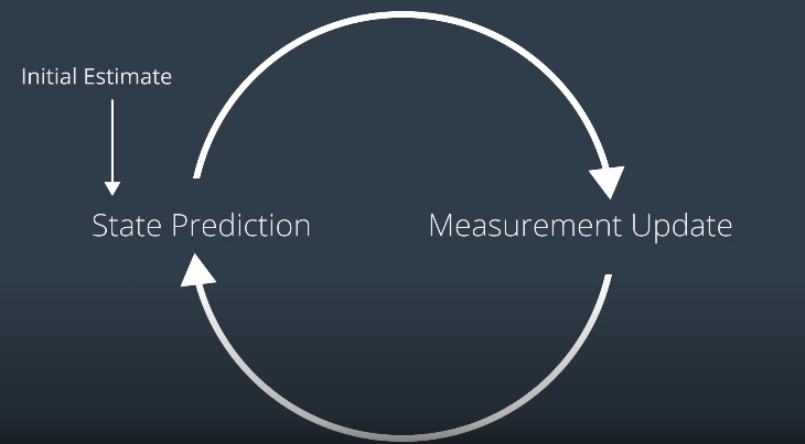
Measurement Update
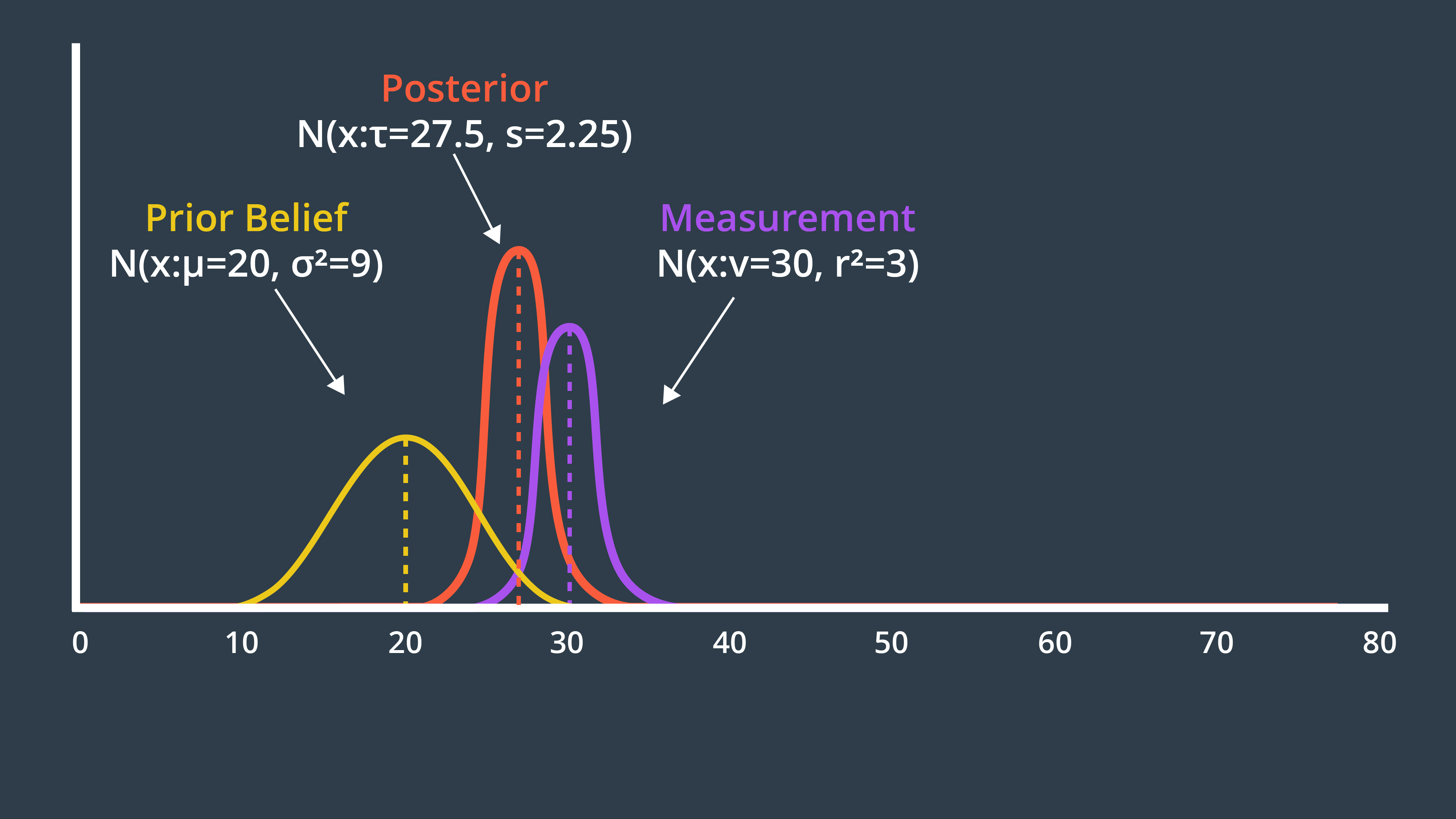
Prior Belief: $\mu_1$ (Mean), $\sigma_1^2$ (Variance)
Measurement: $\mu_2$ (Mean), $\sigma_2^2$ (Variance)
Posterior Belief:
$\mu = \frac{\sigma_2^2}{\sigma_1^2+\sigma_2^2}\mu_1 + \frac{\sigma_1^2}{\sigma_1^2+\sigma_2^2}\mu_2$
- Because $\sigma_1^2 > \sigma_2^2$ and $\mu_2$ is real measurement and we need to give it more weight.
$\frac{1}{\sigma^2} = \frac{1}{\sigma_1^2} + \frac{1}{\sigma_2^2}$
- $\sigma^2 < min(\sigma_1^2,\sigma_2^2)$ : our new state estimate is more confident than our prior belief and our measurement
State Prediction
Motion to perform: $\mu_d$ and $\sigma^2_d$
New prior belief from previous Measurement Update step: $\mu_b$ and $\sigma^2_b$
$\mu = \mu_b + \mu_d$
$\sigma^2 = \sigma^2_b + \sigma^2_d$
Multivariate Gaussians
Formulas
Mean: $\mu = \begin{bmatrix}\mu_x \\ \mu_y\end{bmatrix}$
Covariance: $\sum = \begin{bmatrix}\sigma^2_x & \sigma_x\sigma_y \\ \sigma_y\sigma_x & \sigma_y^2\end{bmatrix}$
- $\sigma_x^2$ and $\sigma_y^2$ are variance
- $\sigma_x\sigma_y $ and $ \sigma_y\sigma_x $ are correlation terms
- $\sigma_x\sigma_y == \sigma_y\sigma_x $
- if non-zero, the Gaussian function looks ‘skewed’
Mutivariate Gaussian:
$p(x) = \frac{1}{(2\pi)^\frac{D}{2}|{\sum}|^\frac{1}{2}}e^{-\frac{1}{2}(x-\mu)^T\sum^{-1}(x-\mu)}$
$D$ is dimention. If $D=1$, it is same as 1-D Gaussian formula.
State Prediction
Notation:
- $x’$: predicted next state
- $x$: current state
- $F$: state transition function (cur state -> next state)
- $P’$: predicted next covariance
- $P$: current corvariance
- $Q$: noise
Mean Equation:
- $x’ = Fx$
- For example, an object is moving with constant acceleration:
- $x = \begin{bmatrix}p\\ v\\ a\end{bmatrix}$
- $F = \begin{bmatrix}1&&\Delta{t}&&\frac{1}{2}\Delta{t}^2\\ 0&&1&&\Delta{t}\\ 0&&0&&1\end{bmatrix}$
- $x’ = \begin{bmatrix}p+x\Delta{t}+\frac{1}{2}a\Delta{t}^2\\ v+v\Delta{t}\\ a\end{bmatrix}$
Covariance Equation:
If you multiply the state $x$ by $F$, the covariance will be affect by the square of matrix $F$ ($FF^T$)
- $P’ = FPF^T + Q$
Measurement Update
Notation:
- $z$: measurement (observation)
- $x’$: predicted next state
- $H$: Measurement Function (state -> measurement)
- $H^{-1}$: Measurement Function Inverse (measurement -> state)
- $y$: measurement residual
- $P’$: predicted next covariance
- $S$: used to calculate Kalman Gain
- $R$: measurement noise
Equations:
- $y = z - Hx’$
- $S = HP’H^T+R$
Kalman Gain
Kalman Gain determines how much weight should be place on the state prediction and measurement update (depends on the noise). In other words, it is an averaging factor depending on the uncertainty of the state prediction and measurement update.
Notation:
- $K$: Kalman Gain
- $x$: new current state
- $x’$: predicted next state (predicted new current state)
- $y$: measurement residual
Kalman Gain Equation:
- $K = P’H^TS^{-1}$
Posterior State and Covariance Equation:
- $x = x’ + Ky$
- $P = (I - KH) P’$
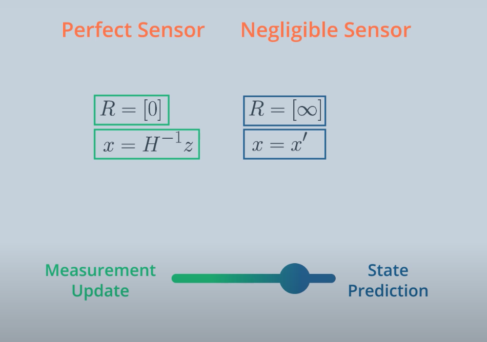
Perfect Measurements Example:
- $R = \begin{bmatrix}0&…&0\\ …&…&…\\ 0&…&0\end{bmatrix} = \begin{bmatrix}0\end{bmatrix}$ (noise = 0 and measurement is 100% accurate)
- $S = HP’H^T+R = HP’H^T$
- $ K = P’H^TS^{-1} = P’H^T(HP’H^T)^{-1} = H^{-1}$
- $x = x’ + Ky = x’ + H^{-1}y = x’ + H^{-1}(z-Hx’) = H^{-1}z$
new_current_state=measurement2state(measurent)In this perfect measurement example, we are only using our measurement to update proterior state.
Negligible Measurements Example:
- $R = \begin{bmatrix}\infty&…&\infty\\ …&…&…\\ \infty&…&\infty\end{bmatrix} = \begin{bmatrix}\infty\end{bmatrix}$ (measurement is not reliable, and uncertainty is as high as possible)
- $S = HP’H^T+R = \begin{bmatrix}\infty\end{bmatrix}$
- $ K = P’H^TS^{-1} = P’H^T(\infty)^{-1} = 0$
- $x = x’ + Ky = x’$
new_current_state=predicted next stateIn this negligible measurement example, the measurement is not included at all because it is unreliable. The posterior state is euqal to state prediction.
Kalman Gain Visulization: determines how much weight between Measurement Update and State Prediction:
Extended Kalman Filter (EKF)
Kalman Filter Assumption:
- Motion and Measurement models are linear
- State space can be represented by a unimodal Gaussian distribution
But, real world problem is non-linear (e.g. move in a circle)
A nonlinear function can be used to update the mean of a function:
- $\mu \xrightarrow{f(x)} \mu’$
To update the variance, the Extended Kalman Filter linearizes the nonlinear function f(x) over a small section and calls it F:
- $P \xrightarrow{F} P’$
The linear approximation can be obtained by using the first two terms of the Taylor Series of the function centered around the mean:
- $F = f(\mu) + \frac{\delta f(\mu)}{\delta x}(x-\mu)$
First two terms of Linearization in Multiple Dimensions Tarlor Series:
- $\large T(x) = f(a) + (x-a)^T\nabla{f(a)}$
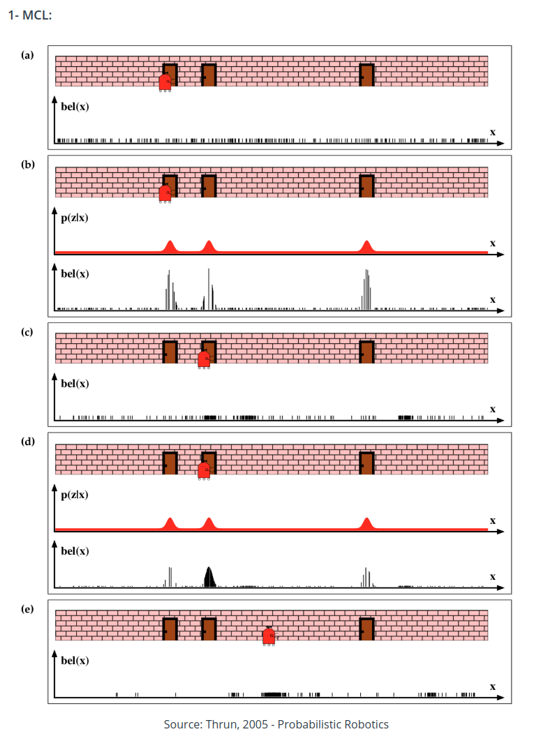
Monte Carlo Localization (MCL)
MCL can only solve Local and Global Localization Problem
Bayes Filters
Robot can estimate the state of a dynamical system from sensor measurements
$Bel(x_t) = P(X_t|Z_{1…t})$
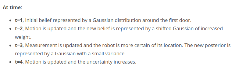
- $Bel$: The probability density, AKA posterior, is called belief
- $X_t$ : State at time t
- $Z_{1…t}$: Measurement
- Recall: $P(A|B) = \frac{P(B|A) * P(A)}{P(B)} = \frac{P(B|A) * P(A)}{P(A) * P(B|A) + P(\neg A) * P(B| \neg A)}$
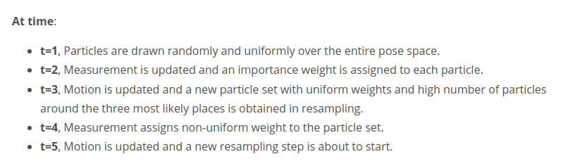
MCL Algorithms
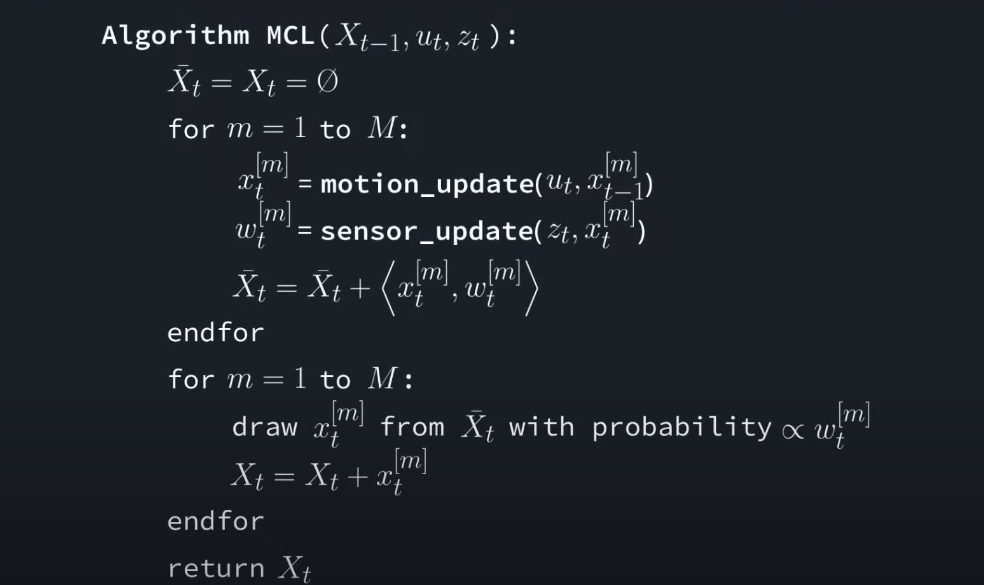
Steps:
- Previous Belief
- Motion Update
- Measurement Update
- Resampling
- New Belief
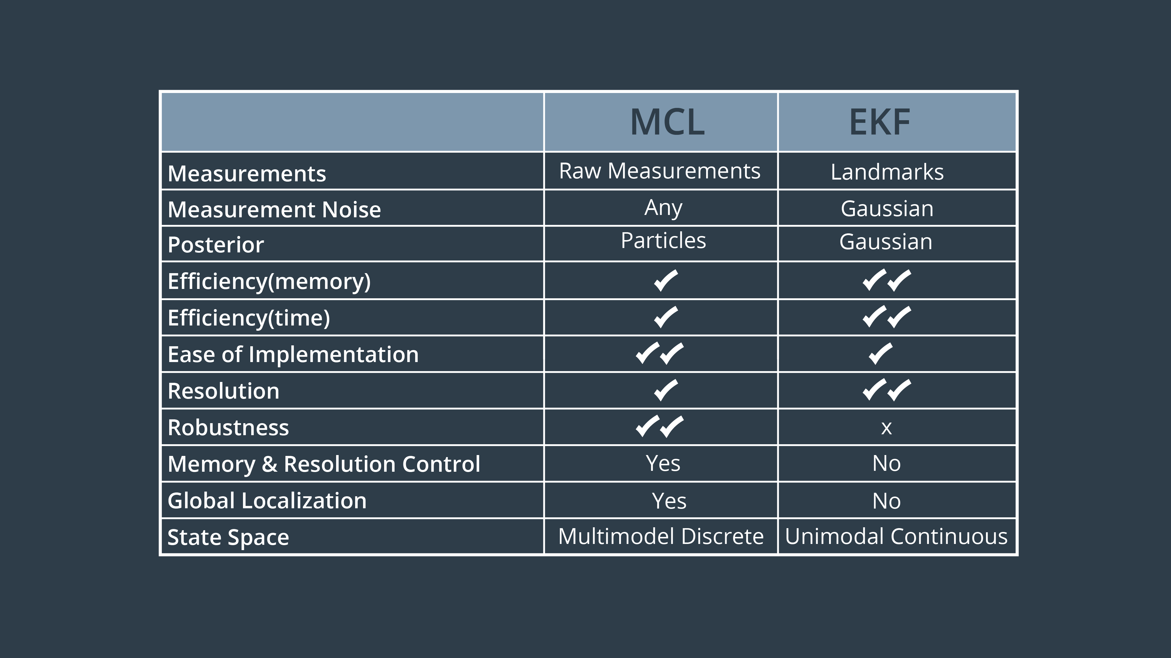
MCL vs EKF
SLAM
SLAM: Simultaneous Localization And Mapping
Localization vs. Mapping
| Localization | Mapping | |
|---|---|---|
| Assumption | Known Map | Robot’s Trajectory |
| Estimation | Robot’s Trajectory | Map |
Occupancy Grid Mapping Algorithm
Discrete Data: the data is obtained by counting. e.g. Number of robots in a room
Continuous Data: the data is obtained by measuring it. e.g., weight of a robot
Notations:
- $x$: estimation
- $z$: measurement
- $m$: map
- $u$: control
| Robotic Problems | Probability Equations |
|---|---|
| Localization | $P(x_{1:t} | u_{1:t}, m, z_{1:t})$ |
| Mapping | $P(m | z_{1:t}, x_{1:t})$ |
| SLAM | $P(x_{1:t}, m | z_{1:t}, u_{1:t})$ |
Forward Measurement Model:
- $P(z_{1:t} | x)$: Estimating a posterior over the measurement given the system state
Inverse Measurement Model:
- $P(x | z_{1:t})$: Estimating a posterior over the system state given the measurement
- Used when measurement is more complex than the system state. e.g. use camera to tell if the door is open
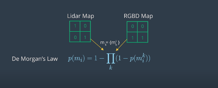
Binary Bayes Filter
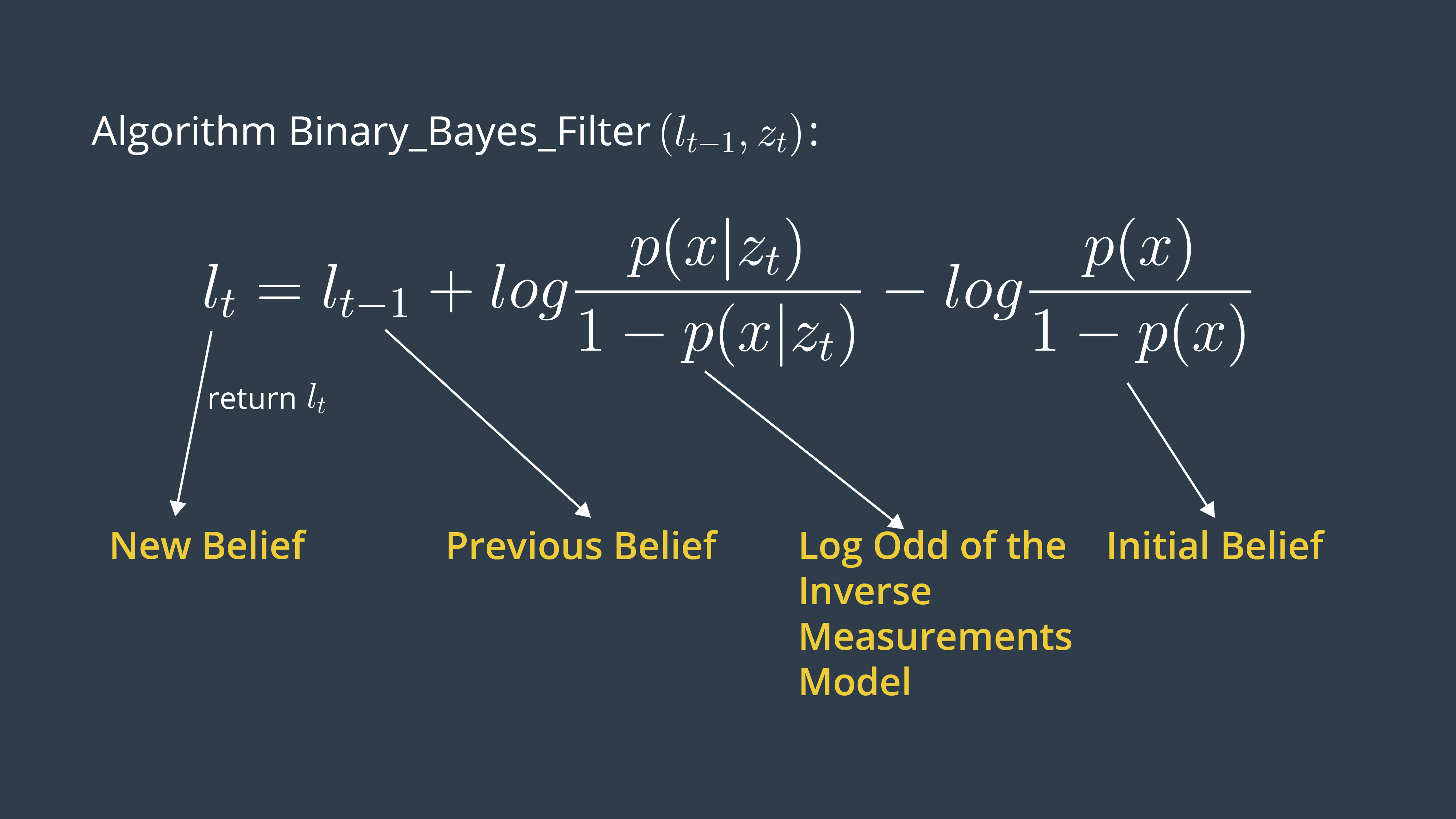
De Morgan’s Law
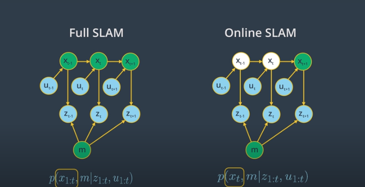
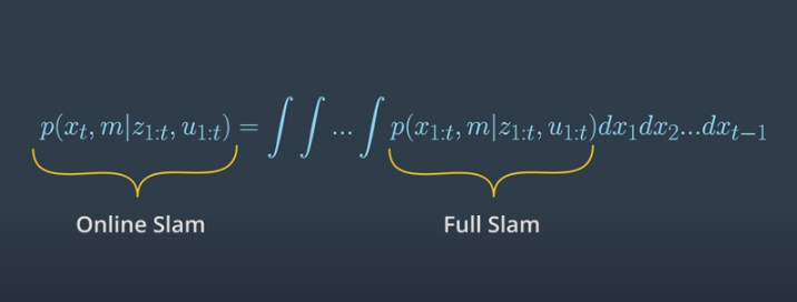
Online SLAM vs Full SLAM
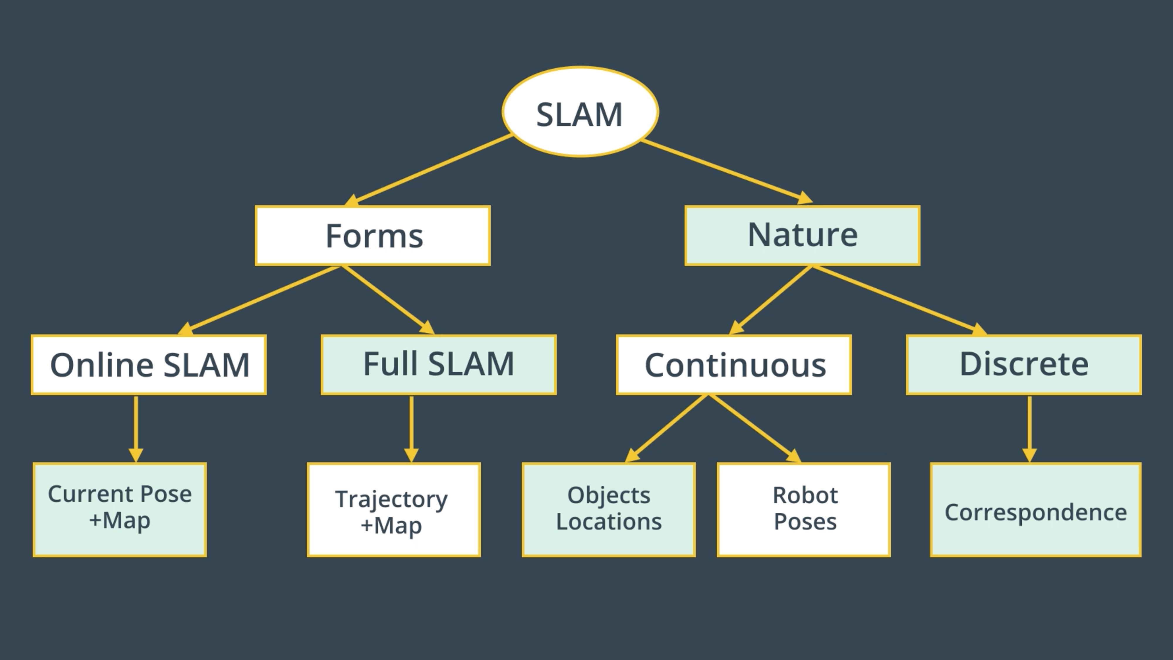
Online SLAM: $P(x_t, m | z_{1:t}, u_{1:t})$
-
Solve the posterior represented by the Instantaneous pose $x_t$ and the map $m$ given all the measurements $z_{1:t}$ and controls $u_{1:t}$
-
with Online SLAM, we estimate variables that occur at time t only
Full SLAM: $P(x_{1:t}, m | z_{1:t}, u_{1:t})$
- Solve the posterior represented by the robot’s trajectory $x_{1:t}$ and the map $m$ given all the measurements $z_{1:t}$ and control $u_{1:t}$
- with Full SLAM. we estimate all the variables that occur throughout the robot travel time
Fast SLAM
FastSLAM algorithm can solve the full SLAM problem with known correspondences with MCL + low-dimensional EKF
Graph SLAM
Maximum Likelihood Estimation (MLE)
-
Probability tries to estimate the outcome given the parameters.
-
Likelihood tries to estimate the parameters that best explain the outcome.
Path Planning
Input:
- Environment Geometry
- Robot Geometry
- Start Pose of Robot
- Goal Pose of Robot
Output:
- Path from start to goal
Discrete Planning
Discretize the workspace into connected graph, then apply a graph-search algo to calculate the best path.

Pros:
- Elegant, Precise, thorough,
- Best suited for low-dim problems
Cons:
- Computationally expensive,
- Not good for high-dim problems
Sample-Based Planning
Takes a number of samples and uses them to build a discrete representation of the ws.

Pros:
- quick
Cons:
- Not precise
Probabilistic Path Planning
Also takes into account the uncertainty of the robot’s motion.
Pros:
- Helpful in highly-contrained environment / env with senstivie and high risk areas
Markov Decision Process
Definition
- A set of states: $S$
- Initial state: $s_0$
- A set of actions: $A$
- The transition model: $T(s, a, s’)$
- A set of rewards: $R$
Solution to a MDP is called policy.
-
Mapping from states to actions
-
An optimal policy: $\pi^*$
Utility of a state:
- $U^\pi(s) = E[\sum_{t=0}^{\infty}R(s_t) | \pi. s_0=s]] = R(s) + U^\pi(s’)$
- $U^\pi(s)$: the utility of a state $s$
- $E$: the expected value
- $R(s)$: the reward for state $s$
- Since the future could be quite uncertain: we will have discounting rate $\gamma^t$ ($\gamma^0=1$)
- $U^\pi(s) = E[\sum_{t=0}^{\infty}\gamma^t R(s_t) | \pi. s_0=s]] = R(s) + U^\pi(s’)$
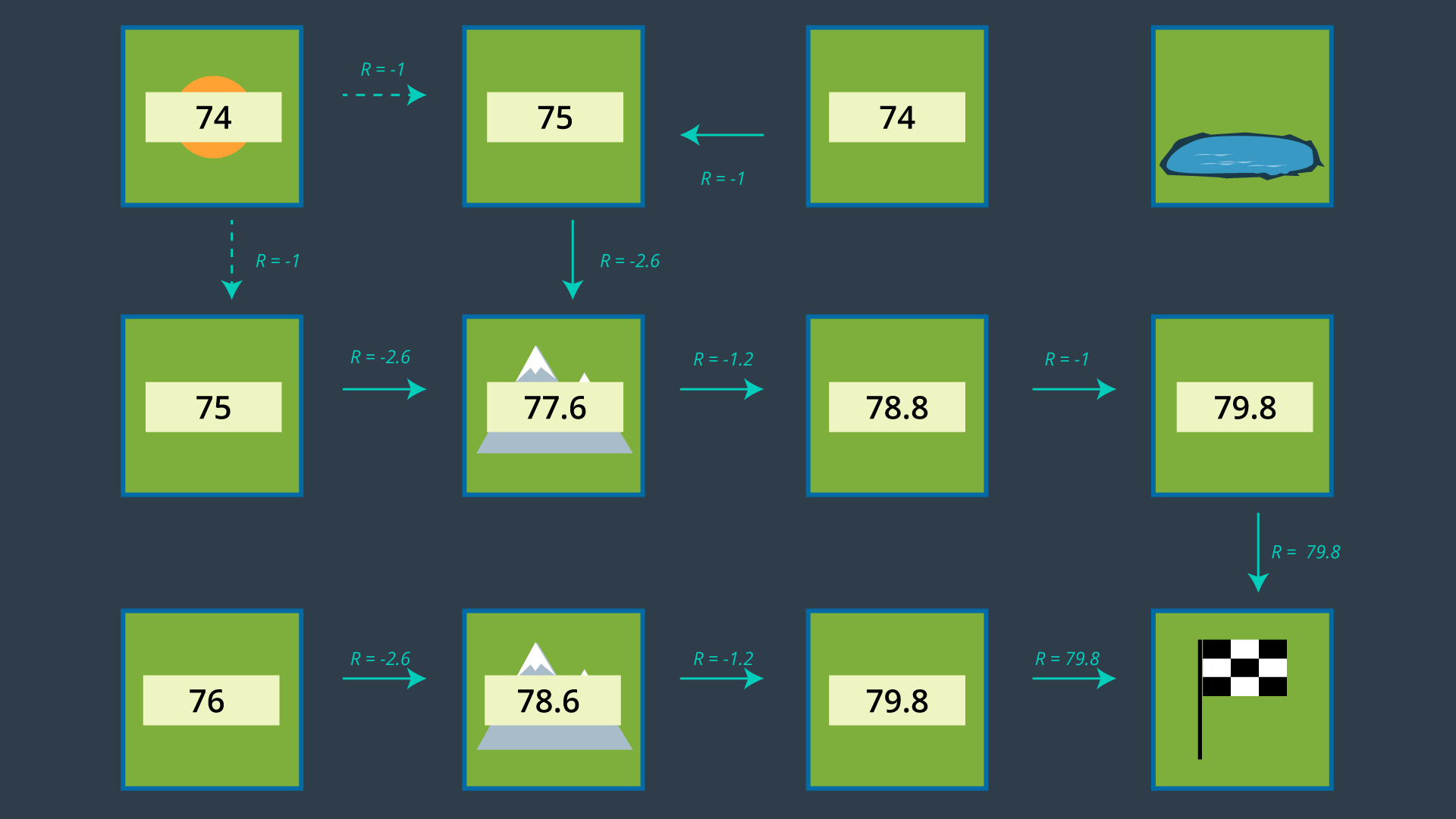
Value Iteration Algorithm
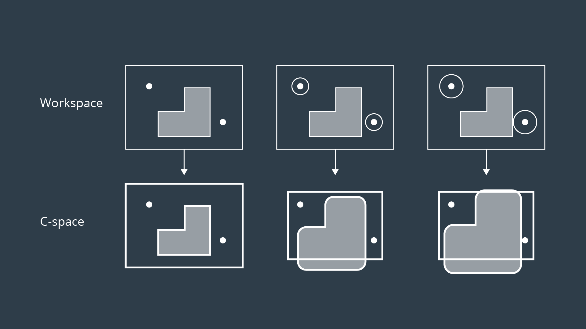
Minkowski Sum
Discretization
- Roadmap
- Cell Decomposition
- Gradient Field
Graph Search
Uninformed Search
- Not provide any info about the the goal
- Example:
- BFS
- DFS
- Uniform Cost Search
Informed Search
-
Provide with info to the goal
-
Example:
- A* Search